Physics-based Deep Learning - Supervised Training

Welcome … — Physics-based Deep Learning

 

 

"지도학습"은 DL의 맥락에서 마주칠 모든 프로젝트의 출발점이며, 따라서 연구할 가치가 있다. 따라서, 좋은 모델 방정식이 존재하지 않는 특정 응용 시나리오에서는 유일한 선택지가 될 수 있다.

 

 

Problem Setting

지도학습의 예로 미지 함수 𝑓*(𝑥) = 𝑦* 를 근사화 하는 과정을 살펴보자

• [𝑥0, 𝑦0], ...[𝑥𝑛, 𝑦𝑛] : 훈련 데이터 (입력 𝑥와 목표 출력 𝑦* 쌍으로 구성)
• f의 가중치 θ를 조정함으로써 손실 함수 최소화
• 즉, 𝑓(𝑥; 𝜃) = 𝑦 ≈ 𝑦* 가 가능한 한 정확하게 되도록 θ 를 제공
• 가장 단순한 L2 Loss로 가정

 

 물리 모델 P를 해결하는 수치 시뮬레이션을 사용하여 훈련을 위한 대량의 신뢰할 수 있는 입력-출력 쌍을 생성하는 것이 이상적이다.

 

 

장점

• 실제 장치의 측정 노이즈가 없음
• 훈련 데이터를 얻기 위해 대량의 샘플에 수동으로 주석을 달 필요가 없음

 

 

주의 사항

• 실제 세계 현상의 행동을 예측할 수 있는 충분한 능력을 갖추고 있는지 확인
• 계산 과정에서 발생하는 오류를 최소화하는 데 주의

 

 

Flow

Surrogate models

 지도 학습 접근 방식의 장점으로는 대체 모델, 즉 원래 P의 행동을 모방하는 새로운 함수를 얻을 수 있다는 점이다. 실제 세계 현상에 대한 PDE 모델의 수치 근사치는 종종 계산하기에 매우 비용이 많이 드는 반면에, 훈련된 NN은 평가당 일정한 비용이 들며, GPU나 NN 유닛과 같은 전문 하드웨어에서 평가하기가 일반적으로 매우 쉽다.

 

 

신경망을 사용할때 고려해야하는 점

• NN(Neural Network)은 엄청난 수의 중간 결과를 빠르게 생성함
• 128개의 특성을 가진 CNN 레이어 구조에서 계산 시 128^2 개의 특성 입력에 대해, 128^3개의 특성 즉, 200만 개 이상의 중간 값들을 생성
• 모든 값들을 메모리에 임시 저장하고 다음 레이어에서 처리하기 때문에 잘 고려해야 함

 

 

Supervised training for RANS flows around airfoils

 지도 학습 예로 Airfoils(날개 프로필) 주위의 난류 공기흐름 상황 가정, RANS 방정식을 해결하기 위한 전통적인 수치 방법에 의존하는 대신, 수치 솔버를 완전히 우회하여 속도와 압력 측면에서 해답을 생성하는 신경망을 통해 대체 모델을 훈련시키는 것을 목표로 본 실습을 진행한다.

 

 

About

• 주요 목표 : 에어포일 주변에서 속도 u = ux, uy와 압력 필드 p를 추론하는 것
• 𝑢𝑥, 𝑢𝑦, 𝑝 : 128^2 차원을 가짐
• Input
  • 레이놀즈 수 : Re ∈ R
  • 공격 각도 : α ∈ R
  • 128^2 의 래스터화된 격자로 인코딩된 Airfoils 모양 s

 

• Output : Airfoils 주변의 속도 필드 u= u_x, u_y, 압력 필드 𝑝
• 상수인 스칼라 입력 Re와 α 역시 128^2의 크기로 확장되어 입출력 모두 x, y^∗ ∈ R^(3×128×128) 동일한 차원을 가짐
• 이때, y∗의 관심 있는 양이 세 가지 다른 물리적 필드를 포함한다는 것을 주의

 

 

RANS training data

import pylab

# helper to show three target channels: normalized, with colormap, side by side
def showSbs(a1,a2, stats=False, bottom="NN Output", top="Reference", title=None):
	c=[]
	
	for i in range(3):
		b = np.flipud( np.concatenate((a2[i],a1[i]),axis=1).transpose())
		min, mean, max = np.min(b), np.mean(b), np.max(b);
		
		if stats:
		 print("Stats %d : "%i + format([min,mean,max]))
		 
		b -= min; b /= (max-min)
		c.append(b)
	
	fig, axes = pylab.subplots(1, 1, figsize=(16, 5))
	axes.set_xticks([]); 
    axes.set_yticks([]);
	im = axes.imshow(np.concatenate(c,axis=1), origin='upper', cmap='magma')
	
	pylab.colorbar(im); pylab.xlabel('p, ux, uy'); pylab.ylabel('%s %s '%(bottom,top))
	if title is not None: 
		pylab.title(title)
	
NUM=72
showSbs(npfile["inputs"][NUM],npfile["targets"][NUM], stats=False, bottom="Target Output", 
				top="Inputs", title="3 inputs are shown at the top (mask, in-ux, in-uy), 
				with the 3 output channels(p,ux,uy) at the bottom")

 

Flow

1. Airfoils 데이터 로드
2. 학습에 필요한 하이퍼 파라미터 정의 ※ Epoch, batch size, learning rate
3. Dataset 정의
4. 데이터 세트에 대한 Dataloar 생성

 

Network setup

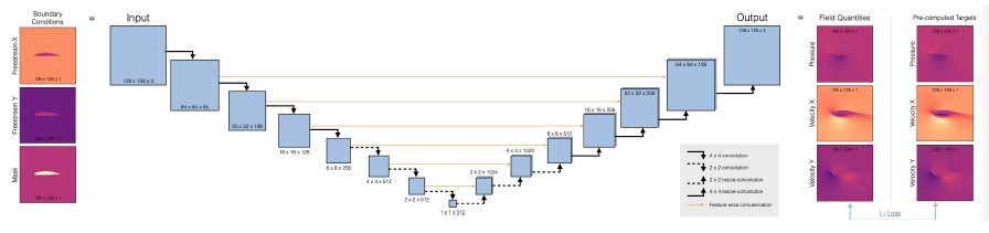
• 신경망의 아키텍처로 전체적으로 합성곱을 사용하는 U-net을 사용
• 일반적인 컨볼루션 네트워크와의 주요 차이점은 인코더부터 디코더 부분까지 Skip-connection을 도입
• 특성 추출 동안 정보가 손실되지 않도록 보장
• 디코더를 독립적인 구성 요소로 사용하고 싶은 경우에는 작동하지 않음
• pooling을 사용하지 않고, strides와 transpose convolutions을 사용

 

 

BlockUNet 함수 정의

import os, sys, random
import numpy as np
import torch
import torch.nn as nn
import torch.optim as optim
import torch.autograd
import torch.utils.data

def blockUNet(in_c, out_c, name, size=4, pad=1, transposed=False, bn=True, activation=True, relu=True, dropout=0. ):
	block = nn.Sequential()
	
	if not transposed:
		block.add_module('%s _conv' % name, nn.Conv2d(in_c, out_c, kernel_size=size, stride=2, padding=pad, bias=True))
	
	else:
		block.add_module('%s _upsam' % name, nn.Upsample(scale_factor=2, mode='bilinear'))
		# reduce kernel size by one for the upsampling (ie decoder part)
		block.add_module('%s _tconv' % name, nn.Conv2d(in_c, out_c, kernel_size=(size-1), stride=1, padding=pad, bias=True))

	if bn:
		block.add_module('%s _bn' % name, nn.BatchNorm2d(out_c))
		
	if dropout > 0.:
		block.add_module('%s _dropout' % name, nn.Dropout2d( dropout, inplace=True))
		
	if activation:
		if relu:
			block.add_module('%s _relu' % name, nn.ReLU(inplace=True))
			
		else:
			block.add_module('%s _leakyrelu' % name, nn.LeakyReLU(0.2, inplace=True))
	
	return block

 

 

DfpNet class 정의

class DfpNet(nn.Module):
	def __init__(self, channelExponent=6, dropout=0.):
		super(DfpNet, self).__init__()
		channels = int(2 ** channelExponent + 0.5)
		
		self.layer1 = blockUNet(3 , channels*1, 'enc_layer1', transposed=False, bn=True, relu=False, dropout=dropout )
		self.layer2 = blockUNet(channels , channels*2, 'enc_layer2', transposed=False, bn=True, relu=False, dropout=dropout )
		self.layer3 = blockUNet(channels*2, channels*2, 'enc_layer3', transposed=False, bn=True, relu=False, dropout=dropout )
		self.layer4 = blockUNet(channels*2, channels*4, 'enc_layer4', transposed=False, bn=True, relu=False, dropout=dropout )
		self.layer5 = blockUNet(channels*4, channels*8, 'enc_layer5', transposed=False, bn=True, relu=False, dropout=dropout )
		self.layer6 = blockUNet(channels*8, channels*8, 'enc_layer6', transposed=False, bn=True, relu=False, dropout=dropout , size=2,pad=0)
		self.layer7 = blockUNet(channels*8, channels*8, 'enc_layer7', transposed=False, bn=True, relu=False, dropout=dropout , size=2,pad=0)
		
		# note, kernel size is internally reduced by one for the decoder part
		self.dlayer7 = blockUNet(channels*8, channels*8, 'dec_layer7', transposed=True, bn=True, relu=True, dropout=dropout , size=2,pad=0)
		self.dlayer6 = blockUNet(channels*16,channels*8, 'dec_layer6', transposed=True, bn=True, relu=True, dropout=dropout , size=2,pad=0)
		self.dlayer5 = blockUNet(channels*16,channels*4, 'dec_layer5', transposed=True, bn=True, relu=True, dropout=dropout )
		self.dlayer4 = blockUNet(channels*8, channels*2, 'dec_layer4', transposed=True, bn=True, relu=True, dropout=dropout )
		self.dlayer3 = blockUNet(channels*4, channels*2, 'dec_layer3', transposed=True, bn=True, relu=True, dropout=dropout )
		self.dlayer2 = blockUNet(channels*4, channels , 'dec_layer2', transposed=True, bn=True, relu=True, dropout=dropout )
		self.dlayer1 = blockUNet(channels*2, 3 , 'dec_layer1', transposed=True, bn=False, activation=False, dropout=dropout )
		

	def forward(self, x):
		# note, this Unet stack could be allocated with a loop, of course...
		out1 = self.layer1(x)
		out2 = self.layer2(out1)
		out3 = self.layer3(out2)
		out4 = self.layer4(out3)
		out5 = self.layer5(out4)
		out6 = self.layer6(out5)
		out7 = self.layer7(out6)
		
		# ... bottleneck ...
		dout6 = self.dlayer7(out7)
		dout6_out6 = torch.cat([dout6, out6], 1)
		dout6 = self.dlayer6(dout6_out6)
		dout6_out5 = torch.cat([dout6, out5], 1)
		dout5 = self.dlayer5(dout6_out5)
		dout5_out4 = torch.cat([dout5, out4], 1)
		dout4 = self.dlayer4(dout5_out4)
		dout4_out3 = torch.cat([dout4, out3], 1)
		dout3 = self.dlayer3(dout4_out3)
		dout3_out2 = torch.cat([dout3, out2], 1)
		dout2 = self.dlayer2(dout3_out2)
		dout2_out1 = torch.cat([dout2, out1], 1)
		dout1 = self.dlayer1(dout2_out1)
		
		return dout1
		
	def weights_init(m):
		classname = m.__class__.__name__
		if classname.find('Conv') != -1:
			m.weight.data.normal_(0.0, 0.02)
			
		elif classname.find('BatchNorm') != -1:
			m.weight.data.normal_(1.0, 0.02)
			m.bias.data.fill_(0)

 

 

DfpNet 인스턴스 초기화

# channel exponent to control network size
EXPO = 3

# setup network
net = DfpNet(channelExponent=EXPO)
#print(net) # to double check the details...

nn_parameters = filter(lambda p: p.requires_grad, net.parameters())
params = sum([np.prod(p.size()) for p in nn_parameters])
# crucial parameter to keep in view: how many parameters do we have?

print("Trainable params: {} -> crucial! always keep in view... ".format(params))

net.apply(weights_init)

criterionL1 = nn.L1Loss()
optimizerG = optim.Adam(net.parameters(), lr=LR, betas=(0.5, 0.999), weight_decay=0.0)

targets = torch.autograd.Variable(torch.FloatTensor(BATCH_SIZE, 3, 128, 128))
inputs = torch.autograd.Variable(torch.FloatTensor(BATCH_SIZE, 3, 128, 128))

 

Training

history_L1 = []
history_L1val = []

if os.path.isfile("network"):
	print("Found existing network, loading & skipping training")
	net.load_state_dict(torch.load("network")) # optionally, load existing network
	
else:
	print("Training from scratch")
	for epoch in range(EPOCHS):
		net.train()
		L1_accum = 0.0
		
		for i, traindata in enumerate(trainLoader, 0):
			inputs_curr, targets_curr = traindata
			inputs.data.copy_(inputs_curr.float())
			targets.data.copy_(targets_curr.float())
			
			net.zero_grad()
			gen_out = net(inputs)
			
			lossL1 = criterionL1(gen_out, targets)
			lossL1.backward()
			optimizerG.step()
			L1_accum += lossL1.item()
		
		# validation
		net.eval()
		L1val_accum = 0.0
		
		for i, validata in enumerate(valiLoader, 0):
			inputs_curr, targets_curr = validata
			inputs.data.copy_(inputs_curr.float())
			targets.data.copy_(targets_curr.float())
			
			outputs = net(inputs)
			outputs_curr = outputs.data.cpu().numpy()
			
			lossL1val = criterionL1(outputs, targets)
			L1val_accum += lossL1val.item()
			
			# data for graph plotting
			history_L1.append( L1_accum / len(trainLoader) )
			history_L1val.append( L1val_accum / len(valiLoader) )
			
			if epoch<3 or epoch%20==0:
				print( "Epoch: {} , L1 train: {:7.5f} , L1 vali: {:7.5f} ".format(epoch, history_L1[-1], history_L1val[-1]) )
	
torch.save(net.state_dict(), "network" )
print("Training done, saved network")

 

 

Result 시각화

import matplotlib.pyplot as plt

l1train = np.asarray(history_L1)
l1vali = np.asarray(history_L1val)

plt.plot(np.arange(l1train.shape[0]),l1train,'b',label='Training loss')
plt.plot(np.arange(l1vali.shape[0] ),l1vali ,'g',label='Validation loss')
plt.legend()
plt.show()

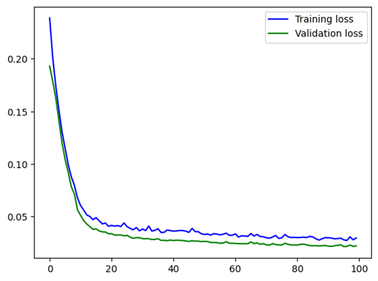
• Validation loss의 초기 값은 약 0.2에서 100회 후 약 0.02로 감소
• 그래프에서 Validation loss가 Training loss보다 낮은 이유는, 훈련 루프의 특성 때문

 

Training progress and validation

net.eval()
for i, validata in enumerate(valiLoader, 0):
	inputs_curr, targets_curr = validata
	inputs.data.copy_(inputs_curr.float())
	targets.data.copy_(targets_curr.float())
	
	outputs = net(inputs)
	outputs_curr = outputs.data.cpu().numpy()
	if i<1: showSbs(targets_curr[0] , outputs_curr[0], title="Validation sample %d "%(i*BATCH_SIZE))

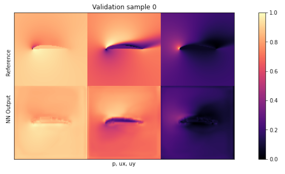
• 훈련 단계 후에 네트워크가 업데이트되어 검증 단계에서는 개선된 상태로 검증 샘플을 처리하기 때문에, 검증 손실이 더 낮게 나올 수 있음

 

 

Test evaluation

• 네트워크를 평가할 때는 훈련 데이터 대신 검증 데이터나 테스트 데이터를 사용해야 과적합을 피할 수 있음을 주의
• 네트워크 훈련 과정에서 훈련하지 않은 새로운 데이터를 사용하여 네트워크의 일반화 능력을 평가

if not os.path.isfile('data-airfoils-test.npz'):
	import urllib.request
	url="<https://physicsbaseddeeplearning.org/data/data_test.npz>"
	print("Downloading test data, this should be fast...")
	urllib.request.urlretrieve(url, 'data-airfoils-test.npz')
	
nptfile=np.load('data-airfoils-test.npz')
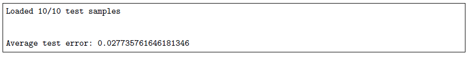
print("Loaded {} /{} test samples\\n".format(len(nptfile["test_inputs"]),len(nptfile["test_targets"])))

testdata = DfpDataset(nptfile["test_inputs"],nptfile["test_targets"])
testLoader = torch.utils.data.DataLoader(testdata, batch_size=1, shuffle=False, drop_last=True)

net.eval()
L1t_accum = 0.
for i, validata in enumerate(testLoader, 0):
	inputs_curr, targets_curr = validata
	inputs.data.copy_(inputs_curr.float())
	targets.data.copy_(targets_curr.float())
	
	outputs = net(inputs)
	outputs_curr = outputs.data.cpu().numpy()
	
	lossL1t = criterionL1(outputs, targets)
	L1t_accum += lossL1t.item()
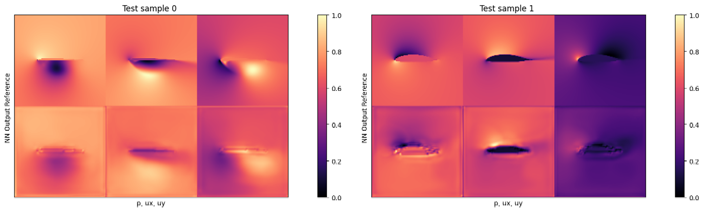
	if i<3: showSbs(targets_curr[0] , outputs_curr[0], title="Test sample %d "%(i))
	
print("\\nAverage test error: {} ".format( L1t_accum/len(testLoader) ))

 

 

Result

• 고압의 정점과 더 큰 y-속도의 포켓이 출력에서 누락 → 네트워크 크기가 작은 이유로 발생
• 평균 테스트 오류는 약 0.03, 즉, 전체 세 필드의 평균 오류 3%

 

→ 그럼에도 매우 복잡한 RANS 솔버를 매우 작고 빠른 신경망 아키텍처로 성공적으로 대체하여 신경망이 복잡한 물리적 모델을 근사할 수 있는 능력을 가지고 있음을 보여줌

 

Discussion of Supervised Approaches

장점

• 레이블이 지정된 데이터를 기반으로 학습하기 때문에 학습이 매우 빠름
• 레이블이 주어지기 때문에 학습이 안정적이고 구현이 상대적으로 간단함
• 딥러닝 모델을 개발할 때 기본적인 성능을 평가하기 좋은 출발점 제공

 

 

단점

• 효과적인 학습을 위해 대량의 데이터가 필요
• 훈련데이터에 과적합될 수 있어, 테스트 데이터에 대해 성능, 정확도 및 일반화가 최적화되지 않을 수 있음
• 외부 프로세스와의 상호 작용이 어려움

 

→ 이러한 supervised training의 단점을 완화하는 방법을 다음 장에서 설명